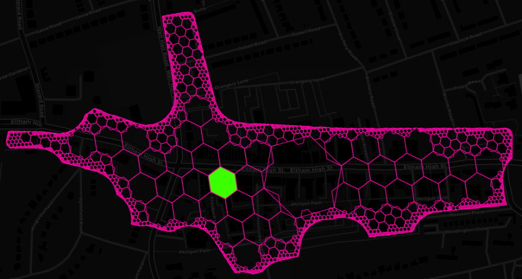
Machine Learning with spatial Big Data: How Uber helped us get there.

There is a notable trend in multinational corporations encouraging their location planners to work more closely with their colleagues in different countries as well as those doing analytics in different departments.

On our end this frequently results in two questions:

Can you do something similar in country X?

and

Can you do something with AI, Machine Learning and Big Data?

So far we could mostly answer these with a confident “yes” (as in mostly “yes”, not mostly confident, as in you only get confident yesses from us or no yesses at all). Artificial intelligence (AI), for one, can be a lot of things and one could claim that good old gravity models exhibit some characteristics consistent with analytical or cognitive intelligence. On the other hand, machine learning algorithms are not traditionally deployed in location planning. One reason for this is that they are more or less opaque. You might get some amazingly accurate predictions with minimal customisation, but do you as an analyst value accuracy and automation more than the ability to track how exactly a forecast came about? Imagine you have an open data source that could give you an indication of where retail is anywhere on the globe – and you might just be happy to sacrifice the latter!

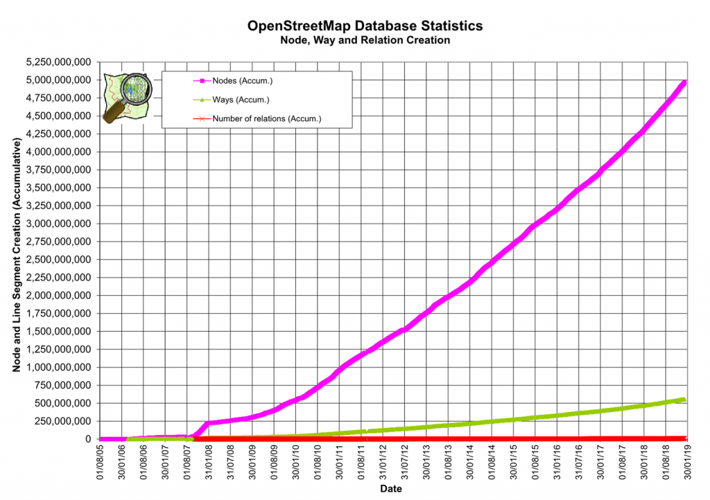
I am, of course, talking about OpenStreetMap (OSM), which to date contains more than five billion features and is steadily growing.

We frequently use OSM to complement other free and proprietary data sets in different countries, but typically face these three major challenges:

1. Coverage: Data density varies across different geographical scales. You might find the amount of data available in a certain country to be very low, but at the same time there is that odd town within, where every tree is mapped along with its species.
2. Semantics: Even though guidelines for how to tag geographical features exist, people can – and do – call things whatever they want for a variety of reasons: There are different notions of what constitutes e.g. a café in different parts of the world, tagging guidelines are community driven and may change over time, and you might even find poor tagging due to ignorance and vandalism.
3. Size: OSM is big. That in itself is not a problem. But the free and open nature of the OSM project means publicly available servers are not meant to cope with large extract requests. In the scenario where you want to extract e.g. 100 retail-related tags for the whole of Europe in one go, you would have to set up the technical infrastructure yourself, along with some decent hardware.

Machine learning, deep learning in particular, offers exciting opportunities to deal with the first two challenges. Rather than adjusting one’s methodology from country to country, region to region, city to city, you could choose to trust, for instance, a neural network to capture the local semantics, given you got some training data across the geography you are interested in. For example, a computer will not scratch its head around why there are so few pubs in Germany – it can be trained to identify the relevance of any tag to any local hub anywhere.

But how do we deal with the sheer size of OSM and get it into shape for the computer to machine learn the hell out of it? – The answer: Call an Uber.

Yes, that was not even first on my list of contrived puns. And yes, I am not referring to a Toyota Prius but one of the many functions that make up H3, the Hexagonal Hierarchical Spatial Index published as open source by the Uber dev team. The idea behind it is beautifully simple. At its core, H3 is nothing more than a global address system – think what3words, minus the fun. You get hexagonal grids at different resolutions and operators to map between these and geographical coordinates.

What makes the real difference though for our Big Data use case, is the ability to interrogate the grid topology and move up and down between resolutions. It allows us to discretise or “bin” OSM features spatially without sacrificing the knowledge of where they are (and where they are in relation to other bins).

This is what the result of the binning process looks like for a hex cell at resolution 11 on the recently redeveloped Eltham High Street (we got a Nando’s!!!):

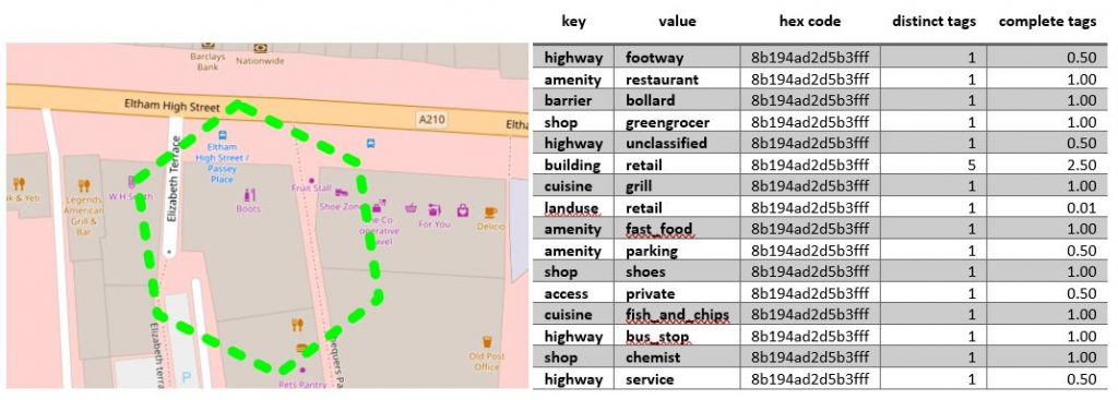
Where “distinct tags” refers to the number of features with that tag intersecting the hex cell and “complete tags” refers to the sum of all inverse cell counts per feature with that tag, which is only relevant for polygon features.

Without going into too much technical detail, it is fair to say achieving the above for the entire OSM data set using actual hex geometries (or of any other shape for that matter) rather than the static (therefore fast) H3 lookups would be a real headscratcher. Conveniently, there are already converters and up-to-date extracts for OSM data into formats suitable for parallel computing. So we could deploy an Apache Spark Scala script utilizing the H3 Java binding on a reasonably sized Google Cloud Dataproc cluster and managed to process the whole lot in less than a day. A PostgreSQL binding for H3 exists and in certain circumstances you might decide a database is the way to go. In this instance, we deemed it more economical to pay for a fast run on throw-away machines and not having to care about hardware and setup.

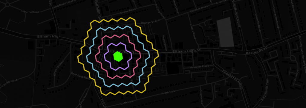
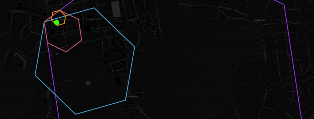
Now, with the above table and some tagged hex cells we can finally start training our machine learning models. While this in itself is a topic for another ten blog posts, I would like to highlight how H3 gives us a great deal of flexibility training these models. In H3 every hex cell “knows” its neighbours and parents, i.e. the bigger hex cells it is contained by. Without going back to the raw data, that is original geometries, we can test model performance on different neighbourhoods and resolutions. We can ask e.g. how significant the occurrence of amenity=bench is to predict retail within the same hex cell or within a distance of 1, 2, 3, 4, … hex cells, or within the same hex cell if that hex cell is 30, 70, 170, … metres across, or both. And we can do that quickly, using simple joins or lookups in a variety of coding environments. The following is a simple example of finding and visualising neighbours and parents using – for the sake of this post – the H3 PostgreSQL binding:

CREATE TABLE example_neighbours AS (
    WITH neighbours AS (
        SELECT k, h3_to_geo_boundary_geometry(h3_k_ring('8b194ad2d5b3fff', k)) AS geom
        FROM generate_series(1, 4) AS t(k)
    )
    SELECT k, ST_Union(geom) AS geom
    FROM neighbours
    GROUP BY k
);

CREATE TABLE example_parents AS (
    SELECT
        res,
        h3_to_parent('8b194ad2d5b3fff', res) AS parent_code,
        h3_to_geo_boundary_geometry(h3_to_parent('8b194ad2d5b3fff', res)) AS geom
    FROM generate_series(7, 10) AS t(res)
);

While in this instance we utilized H3 functions for spatial binning, fast neighbourhood aggregation and resolution reduction, there is a whole lot of other potential applications and this is certainly not the last time you will hear us talking about it. Among the things that spring to my mind are geometry simplification of seamless polygon layers, prettifying polygons with mathematical morphology, building cellular automata like the Game of Life (if you are in that sort of thing) and efficient data transfer (e.g. client-server) through compacting. Compacting is one of these really simple but great ideas. All it does is, given a set of hex codes, to replace higher resolution hex codes with that of the parent as long as all children codes are present. Apart from its potential to greatly reduce the amount of space needed to represent any polygon geometry with a specified level of accuracy, it also makes pretty pictures and is the perfect way to finish this post. Here’s said Eltham High Street from Geolytix’s Retail Places dataset compacted down to submeter accuracy.