European Census and Indices

Everyone knows that census data is an extraordinary rich source of statistical information able to describe a population.

Everyone probably knows that census data can be very complex and, many times, not the most accessible thing in the world. The data can be expensive, it is not always clean, the number of collected variables differs from country to country and their geographical level might vary a lot as well.

This surely doesn’t help people in using it in the easiest possible way and this is why we, at Geolytix, think we created something that might help you out!

Geolytix created and released a free “2011 census pack” for ten European countries (you can find extra information here or you can simply download the data now).

We also created a lifestage and affluence index for 12 different European countries; Austria, Belgium, Ireland, France, Germany, Portugal, UK, Italy, Norway, Spain, Greece and Slovakia.

This year GEOLYTIX have delivered retail network strategy projects across Europe to some of our global clients. These have harnessed our Open European Census data and European Indices. One project for example for a high-end toy retailer, used the census data to identify ‘hotspots’ of children, but also used the disposable income estimates (from the European Indices) to weight the population by affluence. This allowed a more specific target market to be defined as areas of low affluence (at a small geographical level) could be down-weighted reflecting the unlikelihood of these demographic groups to shop at the retailer. This could then be used to score and rank each of the potential locations, helping to form the basis of the network blueprint within each of the markets.

To create our indexes we wanted our input data to be three things:

1.       To be consistent across different countries

2.       To be detailed as much as possible

3.       To relate at a small scale

This means that we invested time in collecting the right data and cleaning it up.

The data that we used came from two different sources: the European Statistical Office (Eurostat) and local data (data published from the government of each single country).

Both have some pros and cons but, the two biggest differences are about consistency and scale. Eurostat data is consistent across all the European countries but relates to a higher geographical level while the other is not consistent but usually relates to the smallest geographical units each country uses for demographic reporting.

Since every country collects census variables differently and that Eurostat uses common variables across Europe, we decided to use Eurostat categories. For this reason, we spent some time in creating a relationship between the two datasets to understand what corresponded to. This was an extremely important step to make because the comparison was not always straightforward. Think of education for example: how different can it be between countries?

To create the lifestage index we considered only two variables, age and population, while for affluence we used the following four categories.

As said before, beside consistency, we also wanted the input data to be detailed as well.

Compared to the local data, which usually collects the population data in age bands, Eurostat is more detailed and it distributes population between 0 and 100 years old. We wanted the same for our input data.

For this reason, we started from lifestage and we distributed the population collected at local level (small scale - table 1) accordingly with the distribution we had in Eurostat (big scale - table 2). As a result (table 3) we had, at a small scale, a highly detailed population (0-100 yo).

For the affluence variables this was a little bit more complicated. Indeed, distributing affluence variables accordingly with the Eurostat distribution might have created new values which didn’t match the population calculated above.

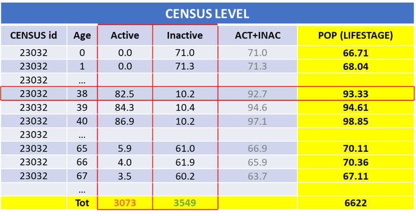
Let’s do an example about two variables of the activity status category, “active” and “inactive” population. The sum of these two variables corresponds to the total population.

If at a local level we had an active and inactive population of respectively, 3,073 and 3,549 people, distributing these values accordingly to Eurostat distribution we got, as a result, the table below. In this, it is possible to see that the sum of the “new” active and inactive values matches the starting values (3,073 and 3,549) but their sum (ACT+INACT) does not match the population value calculated for the lifestage index (POP LIFESTAGE).

This issue was solved using the IPF (iterative proportional fitting procedure) for a bi-dimensional table. This keeps the marginals (POP LIFESTAGE and TOT active & inactive) untouched and moves the values for several loops until the marginal values are hit.

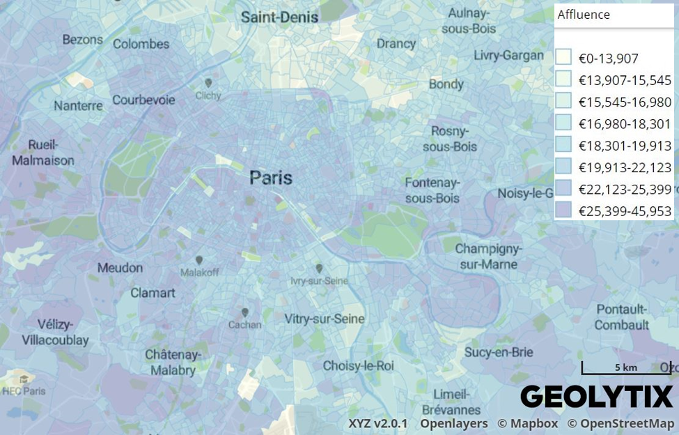
In this map you can see the “Indicators” layer which contains a sample of the results. It refers to the city of Paris, contains just some of the variables used in the index creation and it just refers to the population of 35 years old.

At this point the input data for our indexes was ready and it was consistent, detailed and related to small geographical areas.

The lifestage index was easily done just using a natural break distribution (8 classes) while the affluence one needed more work. In-fact, the input data contained a lot of information and variables and we had to think how to use all this richness.

First thing we did, was to look for something which allowed us to aggregate and to compare our variables. This was the disposable income and then, we aimed to create a regression model to predict the disposable income per person per each census geographical area.

To work with such a high number of variables might generate some problems: it is not always easy to understand the relationship between variables and there is a risk to overfit the model.

One of the possibilities is to try to reduce the number of dimensions dropping some variables. If this allows to create a simpler dataset, on the other hand it has the disadvantage not to gain any information from the dropped variables. Since we didn’t want to delete many variables, dropping only few variables still created a regression model with a huge multicollinearity.

For this reason we decided to use another method: PCA - Principal component analysis. It considers all the variables in the data and it transforms the original variables into a smaller set of linear combinations. This allows us to reduce the number of dimensions without much loss of information. We also tried another method using Tensorflow autoencoders to reduce the dimensionality of the data and it gave back a similar result.

Also here, we create 8 classes for the final index (there is an index calculated at European level and one at country level). You can see the lifestage and the affluence indexes in the map.

Alessandro De Martino, GEOLYTIX